Magnetic Fields due to a Solenoid
A solenoid is made out of a current-carrying wire which is coiled into
a series of turns (with the turns preferably as close together as possible).
The magnetic field due to a
straight length of wire is shown in Figure 1 - the field circles the wire and
its magnitude (or strength) decreases with radial distance from the wire.
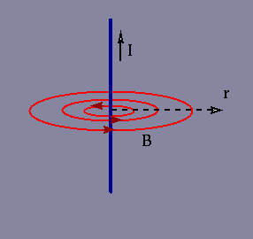
Figure 1: Magnetic field due to a straight wire
In a solenoid, a large field is produced parallel to the axis of the solenoid
(in the z-direction in figure 2).
Components of the magnetic field in other directions are cancelled by
opposing fields from neighbouring coils. Outside the solenoid
the field is also very weak due to this cancellation effect and for a solenoid
which is long in comparison to its diameter, the field is very close to
zero. Inside the solenoid the fields from individual coils add together to
form a very strong field along the center of the solenoid.
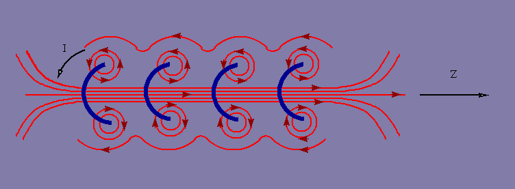
Figure 2: Magnetic field in a solenoid
To calculate the magnitude of the field in the solenoid, we used Ampere's law.
Ampere's law relates the circulation of B around a closed loop to the current
flux through the loop x µ
o.
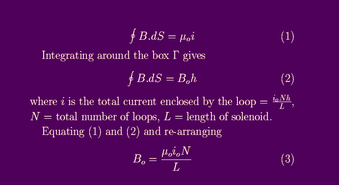
This gives the field in the centre of the solenoid.
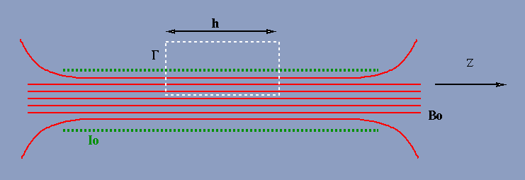
Figure 3: Using Ampere's law to calculate Bo
Note that since the magnitude of the current changes in time, so also
does
Bo, i.e., for a sinusoidally varying current
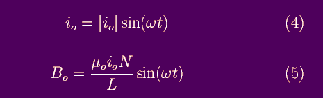
See Figure 4. |B
o| = µ
o i
o N/L is the amplitude (maximum value) of the field.
You can also refer to an "average" value of |B
o|
called, the root-mean-square (RMS) value.
B
RMS = |B
o|/sqrt(2).
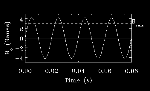
Figure 4: Time-variation of the magnetic field in the solenoid, also showing
BRMS.
However, this doesn't tell you what the field outside the solenoid is.
To calculate this you need to use the Biot-Savart law.
From symmetry, along the z-axis all the components of the field
due to a current loop cancel, except the component in the z-direction.
So
B at a position
z along the axis of the solenoid is given by
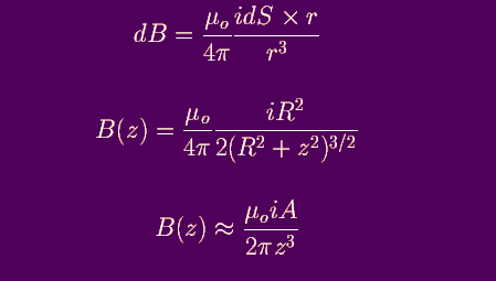 Biot-Savart Law
where R = radius of the loop. The 3rd equation shows B as a function of z when z >> R.
Note that B decreases rapidly as z increases.
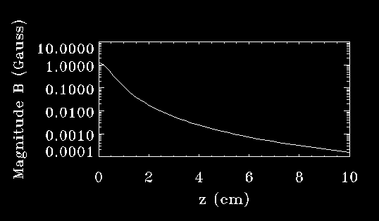
Figure 5: variation of B along the z-axis